almost everything about IMU navigation
strapdown inertial navigation basics with an explanation of IMU pre-integration
Introduction
Inertial Measurement Units (IMU) are ubiquitous devices that are present in many consumer electronic devices today such as smartphones, smart watches, quadrotor drones, vehicles, etc. These are relatively inexpensive and can be a cheap way to know the position and orientation of a device. Their use can range from pedestrian tracking with cheap IMUs to maintaining state for rockets with expensive and accurate IMUs. Therefore, I’ve been fascinated with IMU navigation for a while. In this writeup, I cover the basics required to understand inertial navigation for robot state estimation, and also explain the motivation behind IMU pre-integration
Inertial Measurement Units (IMU) are typically used to track the position and orientation of an object body relative to a known starting position, orientation and velocity. Two configurations of inertial navigation are common
- a stable platform system where the inertial unit is placed in the global coordinate frame and does not move along with the body, and
- a strapdown navigation system where the inertial unit is rigidly attached to the moving object i.e., the IMU is in the body coordinate frame.
These devices typically contain
- Gyroscopes which measure the angular velocity of the body, denoted \({}_b\omega_k\) for angular velocity of the body frame \(b\) at a time instant \(k\)
- Accelerometers which measure the resultant linear acceleration acting on its body, typically denoted with \({}_b a_k\) similarly in the body frame \(b\) at time instant \(k\)
A (micro) micro lie-theory review
An expert reader may choose to skip this section, however this section is important to understand the underlying math and motivation behind IMU pre-integration. This section is largely adapted from Sola et al.
A smooth manifold
is a curved and differentiable (no-spikes / edges) hyper-surface embedded in a higher dimension that locally resembles a linear space \(\mathbb{R}^n\). Examples:
- 3D vectors with unit norm constraint form a spherical manifold in \(\mathbb{R}^3\)
- Rotations in a plane (2D vectors with unit norm constraint) form a circular manifold in \(\mathbb{R}^2\)
- 3D Rotations form a hyper-sphere (3-sphere) in \(\mathbb{R}^4\)
A Group \(\mathcal{G}\)
is a set with a composition operator \(\circ\) that for elements \(\mathcal{X}, \mathcal{Y}, \mathcal{Z} \in \mathcal{G}\) satisfies the following axioms:
- Closure under \(\circ: \mathcal{X} \circ \mathcal{Y} \in \mathcal{G}\)
- Identity \(\mathcal{E}: \mathcal{E} \circ \mathcal{X} = \mathcal{X} \circ \mathcal{E} = \mathcal{X}\)
- Inverse \(\mathcal{X}^{-1}: \mathcal{X}^{-1} \circ \mathcal{X} = \mathcal{X} \circ \mathcal{X}^{-1} = \mathcal{E}\)
- Associativity \((\mathcal{X} \circ \mathcal{Y}) \circ \mathcal{Z} = \mathcal{X} \circ (\mathcal{Y} \circ \mathcal{Z})\) Notice the omission of commutativity
Lie Group
A Lie Group is a smooth manifold that also satisfies the properties of a group. A Lie Group has identical curvature at every point on the manifold (imagine a circle for example).
Some examples:
- \(\mathbb{R}^n\) is a Lie group under the group composition operation of addition.
- The General Linear Real matrix group, the set of all \(n \times n\) invertible matrices \(\mathbb{GL}(n, \mathbb{R}) \subset \mathbb{R}^{n^2}\) is a Lie group under matrix multiplication
- The unit complex number group \(\text{S}^1: \mathbf{z} = \cos \theta + i \sin \theta = e^{i\theta}\) under complex multiplication forms a Lie group. The unit norm of the complex numbers forms a 1-sphere or circle in \(\mathbb{R}^2\)
- The three sphere \(\text{S}^3 \subset \mathbb{R}^4\) is a lie group, we identify with quaternions \(\mathbb{H} \triangleq \{\text{x}_0 + \text{x}_1 i + \text{x}_2 j + \text{x}_3 k \}\) (\(\mathbb{H}\) read as Hamiltonian) under the quaternion multiplication forms a Lie group
2-sphere is not a Lie group
Note that the 2-sphere \(\text{S}^2\) is not a Lie Group, since we cannot define a group composition operator over it. To understand this, let us consider the hairy ball theorem
Lie Group Action
Elements of the Lie group can act on elements from other sets. For example, a unit quaternion \(\mathbf{q} \in \mathbb{H}\) acts on a vector \(\mathbf{x} \in \mathbb{R}^3\) through quaternion multiplication to cause its rotation \(\mathbb{H} \times \mathbb{R}^3 \rightarrow \mathbb{R}^3 : \mathbf{q} \cdot \mathbf{x} \cdot \mathbf{q}^*\).
Tangent space and the Lie Algebra
Let \(\mathcal{X}(t)\) be a point on the Lie manifold \(\mathcal{M}\), then taking its time derivative we obtain \(\dot{\mathcal{X}} = \frac{d\mathcal{X}}{dt}\) which belongs to its tangent space at \(\mathcal{X}\) (or roughly linearized at \(\mathcal{X}\)) denoted as \(T_\mathcal{X}\mathcal{M}\). Since we note that the lie group has the same curvature throughout the manifold, the tangent space \(T_{\mathcal{X}}\mathcal{M}\) also has the same structure everywhere. In fact, by definition every Lie group of dimension \(n\) must have a tangent space described by \(n\) basis elements \(\{\text{E}_1 \dots \text{E}_n\}\) (sometimes also called generators) for \(T_\mathcal{X}\mathcal{M}\).
For instance, the tangent space for the unit complex number group \(\text{S}^1\) is the tangent to a circle at any point forming a straight line i.e., \(\in \mathbb{R}^1\).
The Lie Algebra then is simply the tangent space of a Lie group – linearized – at the identity element \(\mathcal{E}\) of the group. Every Lie group \(\mathcal{M}\) has an associated lie algebra \(\mathfrak{m} \triangleq T_\mathcal{E}\mathcal{M}\). The Lie algebra \(\mathfrak{m}\) is a vector space.
\(\wedge\) and \(\vee\) operators
We can also define functions that convert the tangent space elements between their vector space representation \(\mathbb{R}^m\) and their structured space \(\mathfrak{m}\) using the \(\text{hat}\) and \(\text{vee}\) operators.
- \[\wedge: \mathbb{R}^m \rightarrow \mathfrak{m}; \tau \rightarrow \tau^\wedge = \sum_{i=1}^{m} \tau_i \text{E}_i\]
- \[\vee: \mathfrak{m} \rightarrow \mathbb{R}^m; \tau^{\wedge} \rightarrow (\tau^{\wedge})^{\vee} = \tau = \sum_{i=1}^{m} \tau_i \text{e}_i\]
where let’s signify \(\text{e}_i\) as the basis elements of \(\mathbb{R}^m\). In this article, I will largely attempt to not make use of these operators in an attempt to keep the math concise, and in most cases the variant of Lie algebra used is apparent from context.
\(\mathbf{exp}\) and \(\mathbf{log}\) map
Now, we may define two operators to navigate between Lie group and the Lie algebra as follows:
- \(\text{exp}: T_\mathcal{X}\mathcal{M} \rightarrow \mathcal{M}\) a map that retracts (takes) elements on the tangent vector space to the Lie Group space exactly. Intuitively, the \(\text{exp}\) operator wraps the tangent element onto the Lie group manifold.
- Similarly \(\text{log}: \mathcal{M} \rightarrow T_\mathcal{X}\mathcal{M}\) a map that takes elements on the group to its tangent vector space element.
The \(\text{exp}\) naturally arises when considering the time derivative, or an infinitesimal tangent increment \(v \in T_\mathcal{X}\mathcal{M}\) per unit time on the group manifold:
\(\begin{align} \frac{d\mathcal{X}}{dt} &= \mathcal{X}{v} \\ \frac{d\mathcal{X}}{\mathcal{X}} &= v~dt \\ \text{integrating} \implies \mathcal{X}(t) &= \mathcal{X}(0) \text{exp}(vt) \\ \implies \text{exp}(vt) &= \mathcal{X}(0)^{-1}\mathcal{X}(t) \in \mathcal{M} \end{align}\) i.e., \(\text{exp}(vt)\) is a group element.
Properties of the \(\text{exp}\) map
The \(\text{exp}\) map satisfies a few important properties which are useful to know
- \[\text{exp}((t + s) \tau) = \text{exp}(t \tau) \text{exp}(s \tau)\]
- \[\text{exp}(t\tau) = \text{exp}(\tau)^t\]
- \[\text{exp}(-\tau) = \text{exp}(\tau)^{-1}\]
- \[\begin{align}\text{exp}(\mathcal{X} \tau \mathcal{X}^{-1}) = \mathcal{X} \text{exp}(\tau) \mathcal{X}^{-1} \label{eq:adjoint_property}\end{align}\]
Where the last property is quite important, which I understand as: the exponential map is a no-op for elements already on the Lie manifold
\(\mathbf{SO(3)}\) example
The group of rotations \(\mathbf{SO}(3)\) is a matrix group of size 9 operating on \(\mathbb{R}^3\), with the following constraints:
- It is invertible \(\implies \mathbf{SO(3)} \subseteq \mathbb{GL}(3)\)
- It is orthogonal i.e., it has a determinant of \(\pm\) 1 \(\implies \mathbf{SO}(3) \subseteq \mathbf{O}(3)\)
- It is special orthogonal i.e., determinant is strictly \(+1\) i.e., reflections are not possible.
For this group, we have the special orthogonality condition which can be written as:
\[\mathbf{R}^{-1}\mathbf{R} = \mathbf{I} = \mathbf{R}^\top \mathbf{R}\]since \(\mathbf{R}^{-1} = \mathbf{R}^\top\). Now, to obtain the tangent space for this group, let’s take the time differential of this equation:
\[\begin{align} \dot{\mathbf{R}}^\top \mathbf{R} + \mathbf{R}\dot{\mathbf{R}}^\top &= 0 \\ \implies \dot{\mathbf{R}}^\top \mathbf{R} &= -\mathbf{R}\dot{\mathbf{R}}^\top \\ \implies \dot{\mathbf{R}}^\top \mathbf{R} &= - (\dot{\mathbf{R}}^\top \mathbf{R})^\top \end{align}\]This means that \(\dot{\mathbf{R}}^\top \mathbf{R}\) is skew-symmetric, and skew symmetric matrices always have the following form:
\[[\boldsymbol\omega]_\times = \begin{bmatrix}0 & -\omega_z & \omega_y \\ \omega_z & 0 & -\omega_x \\ -\omega_y & \omega_x & 0\end{bmatrix}\]Therefore we can write \(\dot{\mathbf{R}}^\top \mathbf{R}\) is of the form \([\boldsymbol\omega]_\times\) or
\(\begin{align} \dot{\mathbf{R}} = \mathbf{R}[\boldsymbol\omega]_\times \label{eq:so3_lie_algebra} \end{align}\).
When \(\mathbf{R} = \mathbf{I}\), then \(\dot{\mathbf{R}} = [\boldsymbol\omega]_\times\), which consequently means that \([\boldsymbol\omega]_\times\) the space of skew symmetric matrices forms the Lie algebra for \(\text{SO}(3)\). Finally, we observe that \([\boldsymbol\omega]_\times\) is 3 degrees of freedom by inspection, and that it can be represented as a linear combination of generators as follows:
\[\begin{align} [\boldsymbol\omega]_\times = \omega_x \begin{bmatrix}0 & 0 & 0 \\ 0 & 0 & -1 \\ 0 & 1 & 0\end{bmatrix} + \omega_y\begin{bmatrix} 0 & 0 & 1 \\ 0 & 0 & 0 \\ -1 & 0 & 0\end{bmatrix} + \omega_z \begin{bmatrix}0 & -1 & 0 \\ 1 & 0 & 0 \\ 0 & 0 & 0\end{bmatrix} \label{eq:so3_basis} \end{align}\]if we denote these basis elements as \(\text{E}_x, \text{E}_y, \text{E}_z\) respectively, then we can denote \(\boldsymbol{\omega} = (\omega_x, \omega_y, \omega_z) \in \mathbb{R}^3\) as the vector representation of the lie algebra.
Now, let us attempt to obtain a closed form expression for the \(\text{exp}\) map of \(\text{SO}(3)\). We see from equation (\(\ref{eq:so3_lie_algebra}\)), that we have a differential equation, where \(\dot{\mathbf{R}} = \mathbf{R} [\boldsymbol{\omega}]_\times \in T_\mathbf{R}\text{SO}(3)\). For infinitesimal time increments \(\Delta t\), we can assume that \(\omega\) is constant, then we obtain the solution to the ordinary differential equation as:
\[\begin{align} \int \dot{\mathbf{R}} &= \int \mathbf{R}[\boldsymbol\omega]_\times \Delta t \\ \implies \mathbf{R}(t) &= \mathbf{R}_{0} \text{exp}([\boldsymbol\omega]_\times \Delta t) \end{align}\]If we start at the origin \(\mathbf{R}_0 = \mathbf{I}\), then we have \(\mathbf{R}(t) = \text{exp}([\boldsymbol{\omega}]_\times \Delta t)\).
Now since \(\boldsymbol\omega\) can also be represented as a vector element (see equation (\(\ref{eq:so3_basis}\))), we can define \(\boldsymbol{\theta} \triangleq \omega \Delta t = \mathbf{u} \theta \in \mathbb{R}^3\), where \(\mathbf{u}\) is a unit vector denoting the axis of rotation, and \(\boldsymbol\theta\) denotes the rotation about said axis. It must be noted that 3-axis gyroscopes measure this angular velocity \(\omega\).
Let us now expand the matrix exponential terms:
\[\begin{align} \mathbf{R} = \text{exp}([\boldsymbol\theta]_\times) = \sum_k \frac{\theta^k}{k !}([\mathbf{u}]_\times)^k \end{align}\]Using the properties of skew symmetric matrices we see that \([\mathbf{u}]^0_\times = \mathbf{I}, [\mathbf{u}]^3_\times = -[\mathbf{u}]_\times, [\mathbf{u}]^3_\times = -[\mathbf{u}]^2_\times\). We can thus rewrite the series above as
\[\begin{align} \mathbf{R} &= \mathbf{I} + [\mathbf{u}]_\times \Bigl\{ \theta - \frac{1}{3!}\theta^3 + \frac{1}{5!}\theta^5 - \dots \Bigr\} + [\mathbf{u}]_\times^2 \Bigl\{ \frac{1}{2} \theta^2 - \frac{1}{4!}\theta^4 + \frac{1}{6!}\theta^6 -\dots \Bigr\} \\ \mathbf{R} &= \mathbf{I} + [\mathbf{u}]_\times \sin \theta + [\mathbf{u}]^2_\times (1 - \cos \theta) \label{eq:rodrigues} \end{align}\]Where equation (\(\ref{eq:rodrigues}\)) is the closed form expression for the exponential map for \(\text{SO}(3)\) and also known as the rodrigues formula
\(\oplus\), \(\ominus\) and the Adjoint operators
\(\oplus\) and \(\ominus\) operators allow us to define increments on the Lie group. These combine the composition operator and the \(\text{exp}\) and \(\text{log}\) operator together. Because the composition operation on Lie groups is not commutative, we obtain two variants, \(\text{right}\) and \(\text{left}\) operators
\[\begin{align} \text{right}~\oplus &: \mathcal{Y} = \mathcal{X} \oplus {}^\mathcal{X}\tau \triangleq \mathcal{X} \circ \text{exp}({}^\mathcal{X}\tau^\wedge) \in \mathcal{M} \label{eq:right_oplus}\\ \text{right}~\ominus &: {}^\mathcal{X}\tau = \mathcal{Y} \ominus \mathcal{X} \triangleq \text{log}(\mathcal{X}^{-1}\circ \mathcal{Y})^\vee \in T_\mathcal{X}\mathcal{M} \end{align}\]Notice that in the above operator \(\exp({}^\mathcal{X}\tau^\wedge)\) appears on the right side of the composition \(\circ\) operator. Note that \({}^\mathcal{X}\) denotes that the tangent element is linearized at \(\mathcal{X}\) Similarly we have the \(\text{left}\) variants of the operators which include Lie algebra increments instead:
\[\begin{align} \text{left}~\oplus &: \mathcal{Y} = {}^\mathcal{E}\tau \oplus \mathcal{X} \triangleq \text{exp}({}^\mathcal{E}\tau^\wedge) \circ \mathcal{X} \in \mathcal{M} \label{eq:left_oplus}\\ \text{left}~\ominus &: {}^\mathcal{X}\tau = \mathcal{Y} \ominus \mathcal{X} \triangleq \text{log}(\mathcal{Y} \circ \mathcal{X}^{-1})^\vee \in T_\mathcal{E}\mathcal{M} \end{align}\] While there is a clear distinction in the operand order for right and left \(\oplus\) operator, the \(\ominus\) operator is quite ambiguous. Figure \(\ref{fig:oplus_ominus}\) illustrates the order of operations on a manifold.
Now, if we observe that when traversing on the Lie group one can reach an element \(\mathcal{Y} \in \mathcal{M}\) via two different trajectories as in equation (\(\ref{eq:right_oplus}, \ref{eq:left_oplus}\)), we obtain the following:
\[\begin{align} \mathcal{Y} = \mathcal{X} \oplus {}^\mathcal{X}\tau &= {}^\mathcal{E}\tau \oplus \mathcal{X} \\ \text{exp}({}^\mathcal{E}\tau^\wedge) \circ \mathcal{X} &= \mathcal{X} \circ \text{exp}({}^\mathcal{X}\tau^\wedge) \\ \text{exp}({}^\mathcal{E}\tau^\wedge) &= \mathcal{X} \circ \text{exp}({}^\mathcal{X}\tau^\wedge) \circ \mathcal{X}^{-1} \\ &= \text{exp}(\mathcal{X} {}^\mathcal{X}\tau^\wedge \mathcal{X}^{-1})~~~\text{Using property of exp map \ref{eq:adjoint_property}} \\ \implies {}^\mathcal{E}\tau^\wedge = \mathcal{X} {}^\mathcal{X}\tau^\wedge \mathcal{X}^{-1} \label{eq:adjoint} \end{align}\]Equation \(\ref{eq:adjoint}\) can be used to convert a tangent element linearized at a point \(\mathcal{X}\) on the Lie group to the Lie algebra quite easily, this operation is called as the adjoint operator:
\[\text{Ad}_\mathcal{X}: \mathfrak{m} \rightarrow \mathfrak{m}; \tau^\wedge = \text{Ad}_\mathcal{X}(\tau^\wedge) = \mathcal{X} \tau^\wedge \mathcal{X}^{-1}.\]The adjoint operator is quite heavily utilized to obtain some of the IMU pre-integration results, and therefore is quite important to understand.
Navigation with ideal IMU measurements
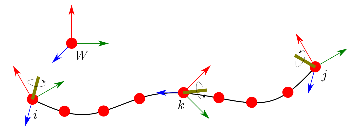
As eluded to in the Introduction, an ideal Inertial Measurement Unit (IMU) mainly contains two sensors Gyroscope and Accelerometer and sometimes optionally a magnetometer. To understand navigation with IMUs, let us first consider an ideal IMU, that can make ideal measurements accurately and precisely, without any noise. Let us specifically consider its operation in a time window between \(i\) and \(j\), and denote any arbitrary time instant within this window as \(k\). The IMU is traveling along a trajectory in the specified time window and it is both rotating and translating in space. An illustration is given in Figure 1.
Gyroscope and inertial orientation
Let us first consider the rotation of the device. An ideal gyroscope measures the angular velocity or how quickly an object is rotating about an axis, as \({}_b \omega_k\) in the body frame \(b\) and time \(k\).
In Figure 1, as the IMU travels along the trajectory from \(i\) to \(j\), the axis of rotation changes continuously. On discretizing the time window and making the piece-wise linear approximation, we can assume that the axis of rotation remains fixed between two timesteps. Then for an instantaneous angular velocity measurement \(\boldsymbol\omega_k\) at time \(k\), the total angular change in rotation is \(\omega_k \Delta t_k^{k+1} \in \mathfrak{so}(3)\). Subsequently we can obtain the relative rotation for the time period \(k\) and \(k+1\) using the exponential map as follows: \(\Delta\mathbf{R}_k^{k+1} = \text{Exp}(\omega_k \Delta t_k^{k+1})\).
Now assuming that the discretization \(\Delta t\) is equal, we can then compose the rotational changes between each \(\Delta t\):
\[\begin{align} {}_W \mathbf{R}_j &= {}_W \mathbf{R}_i \text{Exp}(\omega_i \Delta t_i) \dots \text{Exp}(\omega_k \Delta t_k)\dots \text{Exp}(\omega_j \Delta t_j) \\ \implies {}_W \mathbf{R}_j &= {}_W \mathbf{R}_i \prod_{k=i}^{j}\text{Exp}(\omega_k \Delta t_k) \end{align}\]Accelerometer and inertial velocity and position
Similarly, the accelerometer measures the resultant linear acceleration applied on the robot body. This typically includes any external acceleration that is applied on the body \({}_b \mathbf{a}_k\) and the acceleration due to gravity on the body \((\mathbf{R}_k^W)^\top {}_W \mathbf{g}\). Therefore the total measurement made by an accelerometer is \({}_b \mathbf{a}_k + (\mathbf{R}_k^W)^\top {}_W \mathbf{g}\)
Gravity convention
We understand from highschool physics that an object at rest experiences a normal force equal and opposite to the gravitational force in the world frame \(-{}_W \mathbf{g}\). TODO
Given the initial velocity of the object at \(i\), we can compute the final velocity of the IMU at \(j\) by integrating the instantaneous acceleration measurements \({}_b \mathbf{a}_k\) over the time differences in a similar fashion as for orientation:
\[\begin{align} \mathbf{v}_j = \mathbf{v}_i + \sum_{k=i}^{j-1} \mathbf{R}_b^W(({}_b\mathbf{a}_k + (\mathbf{R}_b^W)^\top {}_W \mathbf{g})\Delta t_k) \\ \mathbf{v}_j = \mathbf{v}_i + {}_W \mathbf{g} \Delta t_i^j + \sum_{k=i}^{j-1} \mathbf{R}_b^W(({}_b\mathbf{a}_k)\Delta t_k \\ \end{align}\]Then, to obtain the position of the body at time \(j\) we need to integrate the velocities at each time instants \(k\) accordingly as below:
\[\]Navigation with real IMU measurements
Why do we care about pre-integration?
Bias estimation and IMU initialization
If you found this useful, please cite this as:
Sharma, Akash (Jul 2024). almost everything about IMU navigation. https://akashsharma02.github.io.
or as a BibTeX entry:
@article{sharma2024almost-everything-about-imu-navigation,
  title   = {almost everything about IMU navigation},
  author  = {Sharma, Akash},
  year    = {2024},
  month   = {Jul},
  url     = {https://akashsharma02.github.io/blog/2024/imu-navigation/}
}